Introduction
In the evidence-based practice of ophthalmology, we often read systematic reviews. Why do we bother about systematic reviews? In science, new findings are built cumulatively on multiple and repeatable experiments [1]. In clinical research, rarely is one study definitive. Using a comprehensive and cumulative approach, systematic reviews synthesize results of individual studies to address a focused question that can guide important decisions, when well-conducted and current [2,3,4,5].
A systematic review may or may not include a meta-analysis, which provides a statistical approach to quantitatively combine results of studies eligible for a systematic review topic [2,3,4,5]. Such pooling also improves precision [2, 4, 5]. A “forest plot” is a form of graphical result presentation [2, 4]. In this editorial, we start with introducing the anatomy of a forest plot and present 5 tips for understanding the results of a meta-analysis.
Anatomy of a forest plot
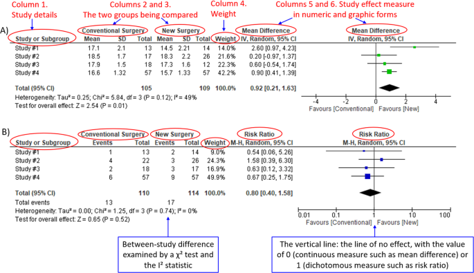
We demonstrate the components of a typical forest plot in Fig. 1, using a topic from a recently published systematic review [6] but replaced with mockup numbers in analysis. In this example, four randomized trials (Studies #1 to #4) are included to compare a new surgical approach with the conventional surgery for patients with pseudoexfoliation glaucoma. Outcomes of intraocular pressure (IOP) and incidence of minor zonulolysis are evaluated at 1-year follow-up after surgery.
A Example of a continuous outcome measure: Intraocular pressure assessed with mean difference; B Example of a dichotomous outcome measure: Incidence of minor zonulolysis, at 1 year after surgery. Tau, the estimated standard deviation of underlying effects across studies (Tau2 is only displayed in the random model). Chi2, the value of Chi-square test for heterogeneity. Random, random model (an analysis model in meta-analysis).
In a forest plot, the box in the middle of each horizontal line (confidence interval, CI) represents the point estimate of the effect for a single study. The size of the box is proportional to the weight of the study in relation to the pooled estimate. The diamond represents the overall effect estimate of the meta-analysis. The placement of the center of the diamond on the x-axis represents the point estimate, and the width of the diamond represents the 95% CI around the point estimate of the pooled effect.
Tip 1: Know the type of outcome than
There are differences in a forest plot depending on the type of outcomes. For a continuous outcome, the mean, standard deviation and number of patients are provided in Columns 2 and 3. A mean difference (MD, the absolute difference between the mean scores in the two groups) with its 95% CI is presented in Column 5 (Fig. 1A). Some examples of continuous outcomes include IOP (mmHg), visual acuity in rank values, subfoveal choroidal thickness (μm) and cost.
For a dichotomous outcome, the number of events and number of patients, and a risk ratio (RR), also called relative risk, along with its 95% CI are presented in Columns 2,3 and 5 (Fig. 1B). Examples of dichotomous outcomes include incidence of any adverse events, zonulolysis, capsulotomy and patients’ needing of medication (yes or no).
Tip 2: Understand the weight in a forest plot
Weights (Column 4) are assigned to individual studies according to their contributions to the pooled estimate, by calculating the inverse of the variance of the treatment effect, i.e., one over the square of the standard error. The weight is closely related to a study’s sample size [2]. In our example, Study #4 consisting of the largest sample size of 114 patients (57 in each group) has the greatest weight, 42.2% in IOP result (Figs. 1A) and 49.9% in zonulolysis result (Fig. 1B).
Tip 3: Pay attention to heterogeneity
Heterogeneity represents variation in results that might relate to population, intervention, comparator, outcome measure, risk of bias, study method, healthcare systems and other factors of the individual studies in a meta-analysis [2, 7]. If no important heterogeneity is observed, we can trust the pooled estimate more because most or all the individual studies are telling the same answer [7].
We can identify heterogeneity by visual inspection of similarity of point estimates, overlapping of confidence intervals, and looking at the results of statistical heterogeneity tests outlined at near the bottom of a forest plot [2, 7]. When more similarity of point estimates and more overlapping of confidence intervals are observed, it means less heterogeneity [2, 7]. The P value generated by the Chi-squared test is the probability of the null hypothesis that there is no heterogeneity between studies. When P < 0.10 is shown, we reject this null hypothesis and consider that there is heterogeneity across the studies [2]. P value of 0.10 is typically used for the test of heterogeneity because of the lack of power for the test [2]. The I2 statistic ranging from 0 to 100%, indicates the magnitude of heterogeneity. Greater I2 indicates more heterogeneity. The I2 below 40% may suggest not important heterogeneity; while the I2 over 75% may suggest considerable heterogeneity [2].
For example in Fig. 1A, the point estimate of Study #1 (i.e., the between-group difference of mean IOP, 2.60 mmHg) is different from the point estimates of Studies #2 to #4 (0.20, 0.60 and 0.90 mmHg, respectively). By virtual observation of 95% CI (the horizontal lines), the 95% of Study #1 just partly overlaps with the other studies’. P-value for heterogeneity of 0.12 is relatively small but still >0.05. The I2 of 49% indicates that a moderate heterogeneity may present [2]. In Fig. 1B, the 95% CIs of all the four studies largely overlap. The large P value for heterogeneity of 0.74 and the I2 of 0% both indicate that no important heterogeneity is detected.
Tip 4: Understand subgroups
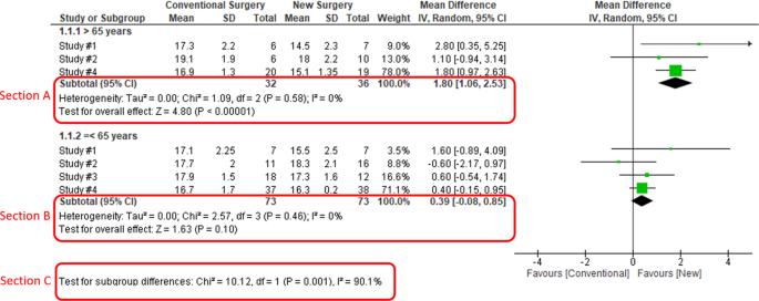
When heterogeneity is detected, which may indicate the unexplained differences between study estimates, using a subgroup analysis is one of the approaches to explain heterogeneity [2]. In our example, Study #3 only studied patients who were equal and below 65 years; Studies #1, 2, and 4 also reported IOP for patients of the two different age groups separately (Fig. 2). We can find the pooled effects of the two subgroups respectively in the forest plot: 1.1.1 over 65 years, the overall effect favours the new surgery (Section A in Fig. 2, subtotal MD and 95% CI does not include the line of no effect, P value for overall effect <0.00001, I2 = 0); and 1.1.2 equal and below 65 years, there is no difference between the conventional and new surgeries (Section B in Fig. 2, subtotal MD and 95% CI includes the line of no effect, P value for overall effect is 0.10, I2 = 0%).
There is a subgroup effect by patients' age groups. We can find the result of test for subgroup difference in the last row of the forest plot (Section C in Fig. 2): P value of 0.001 and I2 of 90.1% indicate a significant difference in treatment effects between the subgroups of patients of older or younger age.
Tip 5: Interpret the results in plain language
In our example, lower IOP and fewer zonulolysis are favoured outcomes. The statistical significance of a pooled estimate can be detected by visual inspection of the diamond (if the diamond width includes the line of no effect, there is no statistical difference between the two groups) or checking the p-value in the last row of a forest plot, “Test for overall effect” (P < 0.05 indicates a significant difference).
In plain language, for patients with pseudoexfoliation glaucoma, the overall effect for IOP is in favour of the new surgery. More specifically, the new surgery is associated with the lower IOP compared to the conventional surgery 1 year after surgery (mean difference, 0.92 mmHg; 95% CI, 0.21 to 1.63 mmHg) with some concerns of heterogeneity and risk of bias. There is no difference in the incidence of minor zonulolysis between new and conventional surgeries.
In summary, knowing the structure of a forest plot, types of outcome measures, heterogeneity and risk of bias assessments will help us to understand the results of a systematic review. With more practice, the readers will gain more confidence in interpreting a forest plot and making application of systematic reviews’ results in your clinical practice.
Change history
08 May 2023
A Correction to this paper has been published: https://doi.org/10.1038/s41433-023-02493-0
References
Zeigler D. Evolution and the cumulative nature of science. Evolution: Education Outreach. 2012;5:585–8. https://doi.org/10.1007/s12052-012-0454-6.
Higgins JP, Thomas J, Chandler J, Cumpston M, Li T, Page MJ, et al. Cochrane handbook for systematic reviews of interventions. John Wiley & Sons; 2019.
Haynes RB. Clinical epidemiology: how to do clinical practice research. Lippincott williams & wilkins; 2012.
Murad MH, Montori VM, Ioannidis JP, Neumann I, Hatala R, Meade MO, et al. Understanding and applying the results of a systematic review and meta-analysis. User’s guides to the medical literature: a manual for evidence-based clinical practice. 3rd edn. New York: JAMA/McGraw-Hill Global. 2015.
Guyatt GH, Oxman AD, Kunz R, Brozek J, Alonso-Coello P, Rind D, et al. GRADE guidelines 6. Rating the quality of evidence—imprecision. J Clin Epidemiol. 2011;64:1283–93. https://doi.org/10.1016/j.jclinepi.2011.01.012.
Pose-Bazarra S, López-Valladares MJ, López-de-Ullibarri I, Azuara-Blanco A. Surgical and laser interventions for pseudoexfoliation glaucoma systematic review of randomized controlled trials. Eye. 2021;35:1551–61. https://doi.org/10.1038/s41433-021-01424-1.
Guyatt GH, Oxman AD, Kunz R, Woodcock J, Brozek J, Helfand M, et al. GRADE guidelines: 7. Rating the quality of evidence—inconsistency. J Clinl Epidemiol. 2011;64:1294–302. https://doi.org/10.1016/j.jclinepi.2011.03.017.
Author information
Authors and Affiliations
Consortia
Contributions
YC was responsible for the conception of idea, writing of manuscript and review of manuscript. MRP was responsible for the conception of idea, and review of the manuscript. VC was responsible for conception of idea, and review of manuscript. MB was responsible for conception of idea, and review of manuscript. RHG was responsible for critical review and feedback on manuscript. LT was responsible for critical review and feedback on manuscript.
Corresponding author
Ethics declarations
Competing interests
YC: Nothing to disclose. MRP: Nothing to disclose. RHG: Advisory boards: Bayer, Novartis, Apellis, Roche, Genentech Inc. LT: Nothing to disclose. MB: Research funds: Pendopharm, Bioventus, Acumed – unrelated to this study. VC: Advisory Board Member: Alcon, Roche, Bayer, Novartis; Grants: Bayer, Novartis – unrelated to this study.
Additional information
Publisher’s note Springer Nature remains neutral with regard to jurisdictional claims in published maps and institutional affiliations.
The original online version of this article was revised: in part 'TIP 4: UNDERSTAND SUBGROUPS', the phrase "In our example, Study #3 only studied patients over 65 years" was corrected to read "In our example, Study #3 only studied patients who were equal and below 65 years".
Rights and permissions
About this article
Cite this article
Chang, Y., Phillips, M.R., Guymer, R.H. et al. The 5 min meta-analysis: understanding how to read and interpret a forest plot. Eye 36, 673–675 (2022). https://doi.org/10.1038/s41433-021-01867-6
Received:
Revised:
Accepted:
Published:
Issue Date:
DOI: https://doi.org/10.1038/s41433-021-01867-6
This article is cited by
-
Estimate the burden of malnutrition among children with cerebral palsy in Sub-Saharan Africa: a systematic review with meta-analysis
Scientific Reports (2024)
-
Surrogate markers of metabolic syndrome and insulin resistance in children and young adults with type 1 diabetes: a systematic review & meta-analysis (MetS and IR in T1DM)
International Journal of Diabetes in Developing Countries (2023)


